Visualize QDF files with VisIt
Visit has a large variety of plots such as pseudocolor plots, vector plots and others. Every plot needs a particular set of data, so it can not plot an arbitrary unknown dataset.
For the QDF data produced by QHG4 we mostly do mesh plots (for meshes and individuals) and pseudocolor plots (for value fields, like environment data).
The example qdf files used here can be found in the subdirectory tutorial_data/example_qdf of the QHG root directory.
When you start VisIt by typing
visit
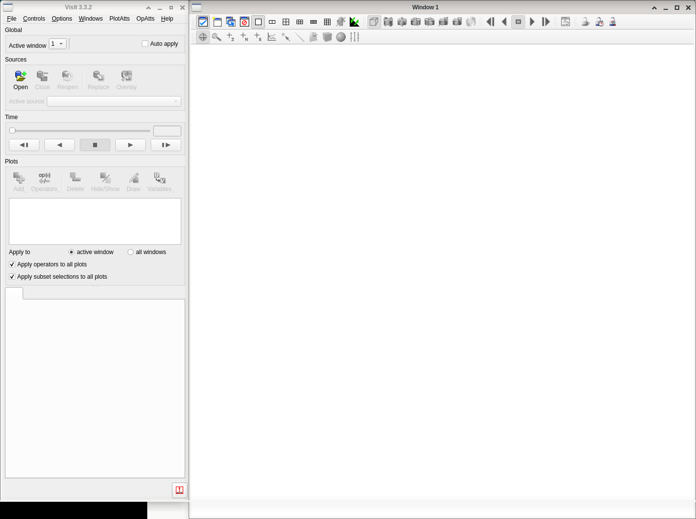
You will see two windows, a control window to the left, and a plot window on the right.
Opening Files
To load a QDF file click on the “Open” button on the upper left of the control window, This will open a file dialog:
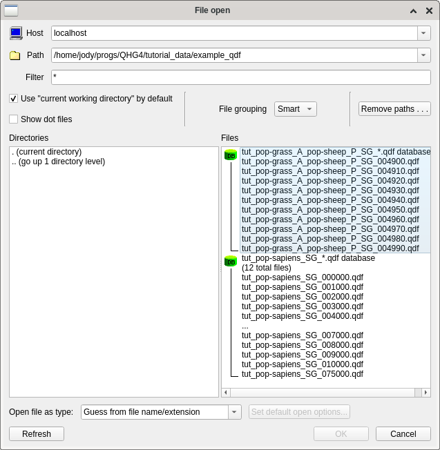
Notice that some files are bundled into groups. VisIt does this to make it possible to load an entire group of similarly named files (e.g. to make an animation or a movie).
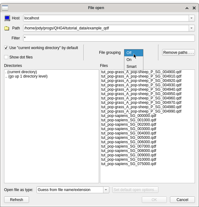
To get rid of the grouping, click on the drop down list “File Grouping” and select “Off”.
Visualizing 2D data
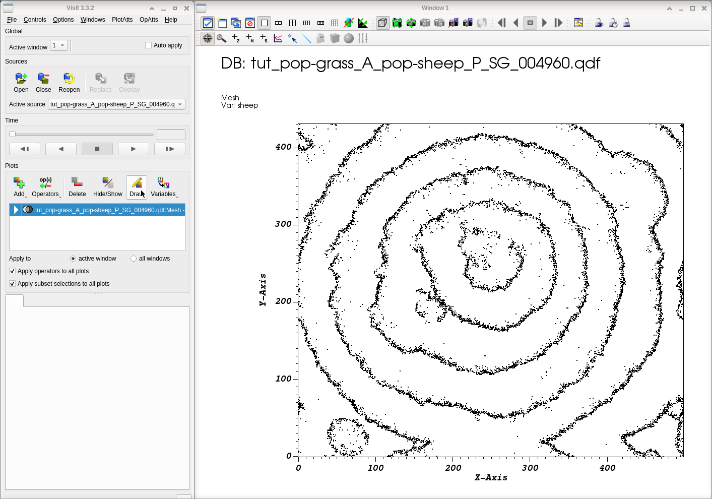
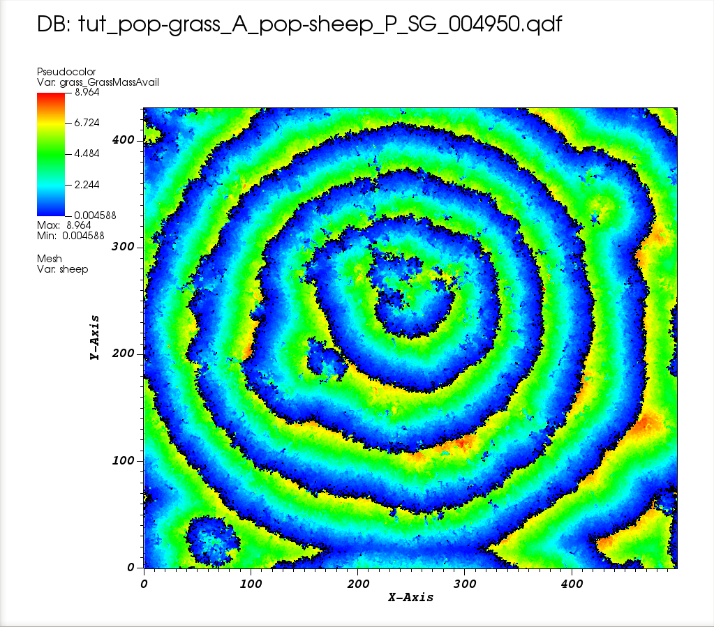
Now select a qdf file containing 2D data by double clicking it, for instance tut_pop-grass_A_pop-sheep-P_SG_004960.qdf (this file comes from a simulation where mobile sheep
eat stationary grass. When there is no grass available in a cell, the sheep will starve unless it finds another cell with grass).
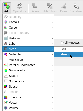
After the file has been loaded, the button “Add” (middle left) in the control dialog becomes active. Clicking this button you see all generally available plots, but not all of them are able to handle QDF data.
To start with, select “Mesh”, and from the pop-up menu choose “Sheep”
If you click on the button “Draw”, you see the sheep agents as black dots.
Next, we add a pseudocolor plot for the available grass: add a pseudocolor plot and select grass_GrasssMassAvail.
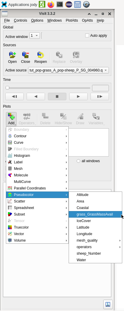
By default, the palette for pseudocolors plots goes from blue (low values) over green to red (high values).
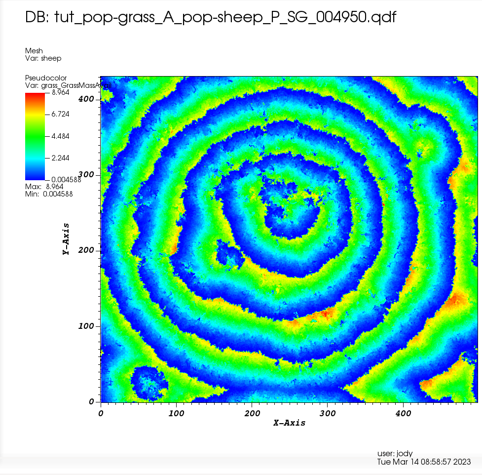
Ater pressing on “Draw”, you’ll notice that the pseudocolor plot is visible, but the sheep have vanished.
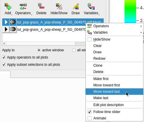
To see both the sheep and the availabla grass, you have to change the order of the plots: Do a right-click on the sheep plot in the dialog’s list, and from there select “Move towards last”
And now enjoy the result:
You can toggle between showing a plot and hiding it by selecting it in the list in the dialog and pressing the button “Hide/Show”. To completely remove a plot, select it and press “Delete”.
Visualizing 3D data
Open a file dialog by pressing “Open”, and if the files appear grouped, ungroup them (see above how to do that).
Then select a 3D data file, such as tut_pop-sapiens_SG_005000.png, press “Add” and select “sapiens” from the submenu of the Mesh plot. and then press “Draw”.
This produces a 3D plot of all agents found in the data. You can rotate the plot by dragging the mouse around the plot window.
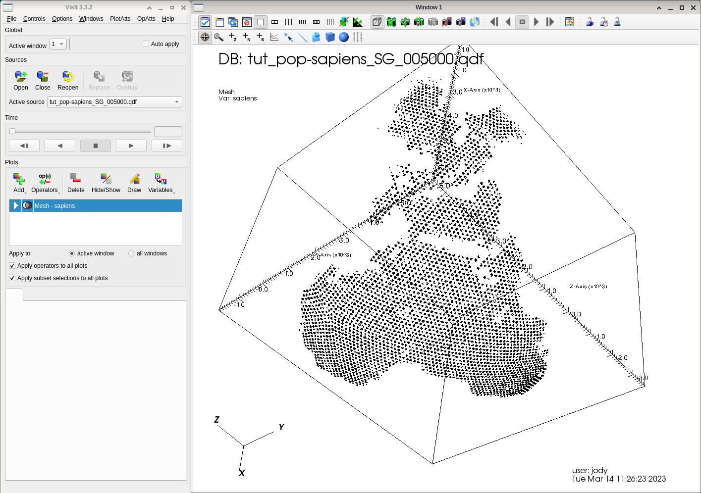
By default VisIt uses a minimal volume encompasssing the loaded data. Since the agents do not cover the entire globe, only a part of the earth is visible.
Let’s change the color of the agents now. Do a double-click on the mesh plot in the list to open the mesh plot attributes.
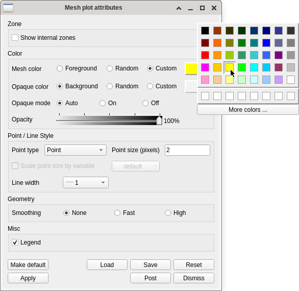
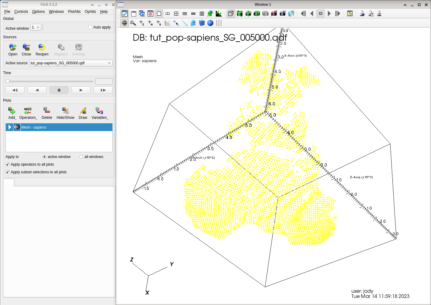
In the upper left of the dialog activate the radio button “Custom” and click on the rectangle beside it. In the small color selector choose a bright color, e.g. yellow, then click on “Apply” in the lower left corner, then “Dismiss” in the lower right corner to hide the dialog.
To plot the earth itself we will use the altitude values.
Click on “Add” and select “Altitude” from the “Pseudocolor” submenu, then press “Draw”.
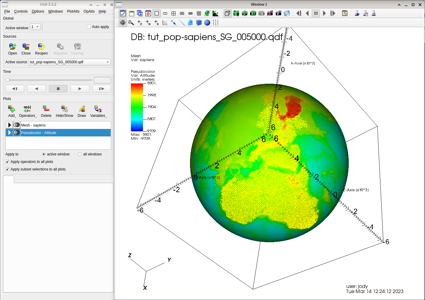
You see a sphere, but it seems the default palette is not very useful here. We’ll use a custom color map created to display altitudes better (see below on how to install it).
So double-click on the Altitude plot in the list.
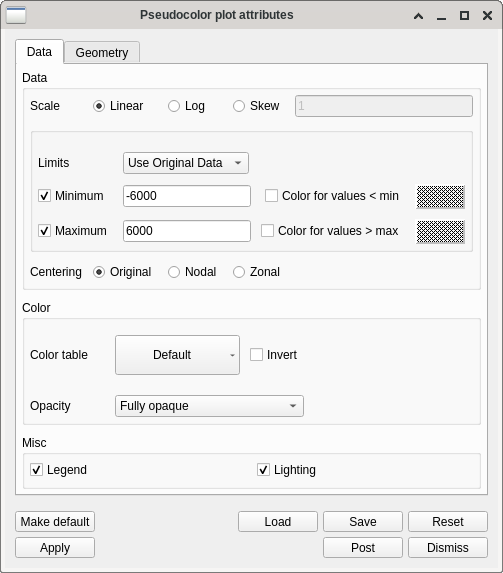
In the plot attribute dialog, set “Minimum” to -6000 and “Maximum” to 6000 (you may have to click the checkboxes to eneble the text fields), and click on the big button in the middle of the dialog (initially this is labeled “Default”). In the pop-up list locate geo2 and click it.
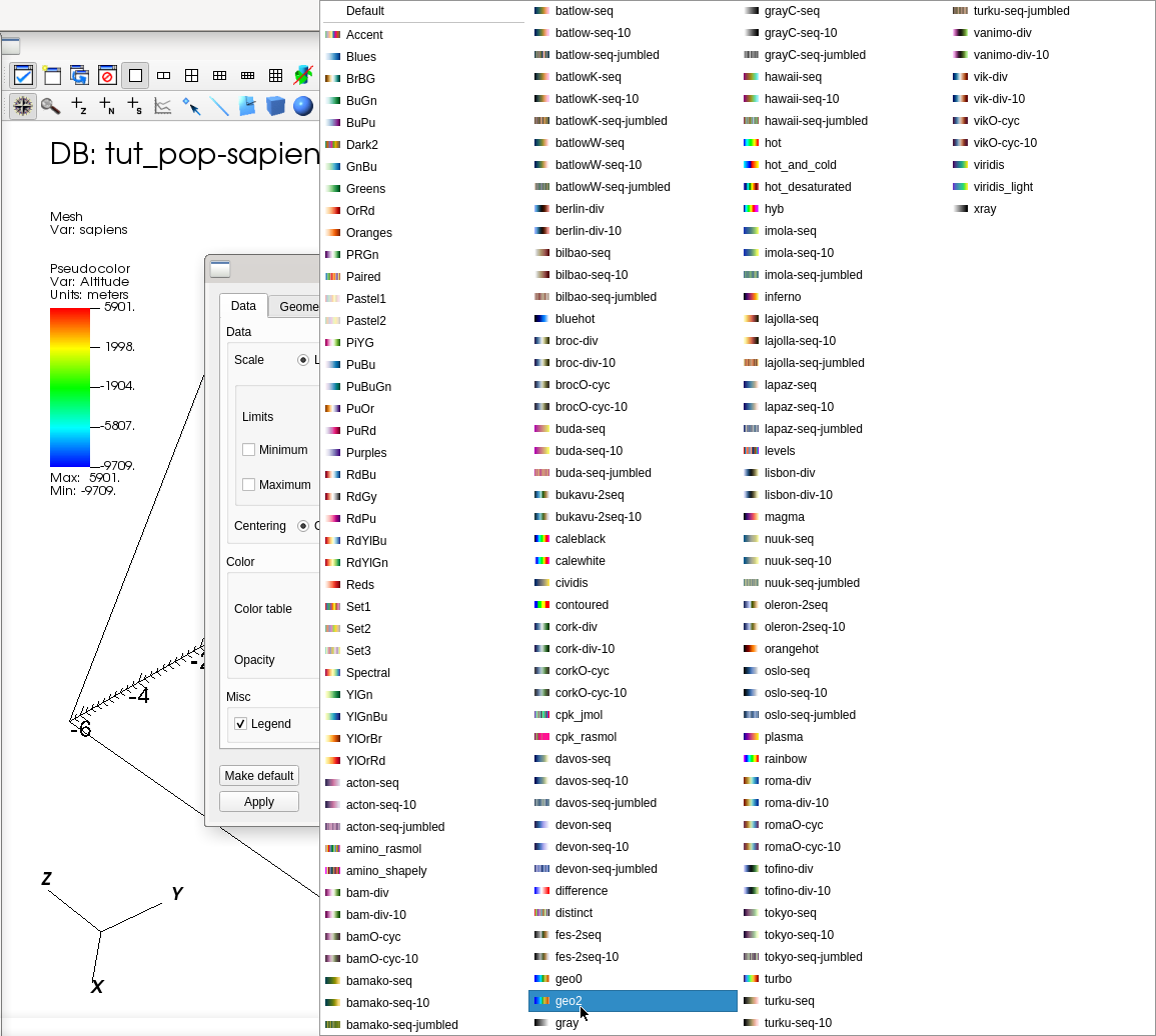
Then press on “Apply” , and “Dismiss” to hide the dialog.
Installing a custom color table
Please consult the color table chapter of the VisIt manual <https://visit-sphinx-github-user-manual.readthedocs.io/en/develop/using_visit/MakingItPretty/Color_tables.html> to get a basic understanding of color tables and how to create, modify, and export them.
When you create and export a color table, visit saves this as a .ct file in the directory``~/.visit``.
The file geo.ct looks like this
<?xml version="1.0"?>
<Object name="ColorTable">
    <Field name="Version" type="string">2.12.3</Field>
    <Object name="ColorControlPointList">
        <Object name="ColorControlPoint">
            <Field name="colors" type="unsignedCharArray" length="4">0 0 255 255 </Field>
        </Object>
        <Object name="ColorControlPoint">
            <Field name="colors" type="unsignedCharArray" length="4">0 0 255 255 </Field>
            <Field name="position" type="float">0.05</Field>
        </Object>
        <Object name="ColorControlPoint">
            <Field name="colors" type="unsignedCharArray" length="4">0 255 255 255 </Field>
            <Field name="position" type="float">0.5i03</Field>
        </Object>
        <Object name="ColorControlPoint">
            <Field name="colors" type="unsignedCharArray" length="4">13 139 0 255 </Field>
            <Field name="position" type="float">0.503</Field>
        </Object>
        <Object name="ColorControlPoint">
            <Field name="colors" type="unsignedCharArray" length="4">203 203 77 255 </Field>
            <Field name="position" type="float">0.6724138</Field>
        </Object>
        <Object name="ColorControlPoint">
            <Field name="colors" type="unsignedCharArray" length="4">216 82 0 255 </Field>
            <Field name="position" type="float">0.95</Field>
        </Object>
        <Object name="ColorControlPoint">
            <Field name="colors" type="unsignedCharArray" length="4">255 255 255 255 </Field>
            <Field name="position" type="float">1</Field>
        </Object>
        <Field name="category" type="string">UserDefined</Field>
    </Object>
</Object>
Obviously this is an xml file.
To install this color table oon your computer, create a file called geo2.ct ,
copy and paste the above text into it, and save it in the directory ~/.visit
(i.e. the (invisible) subdirectory .visit in your home directoryfile).
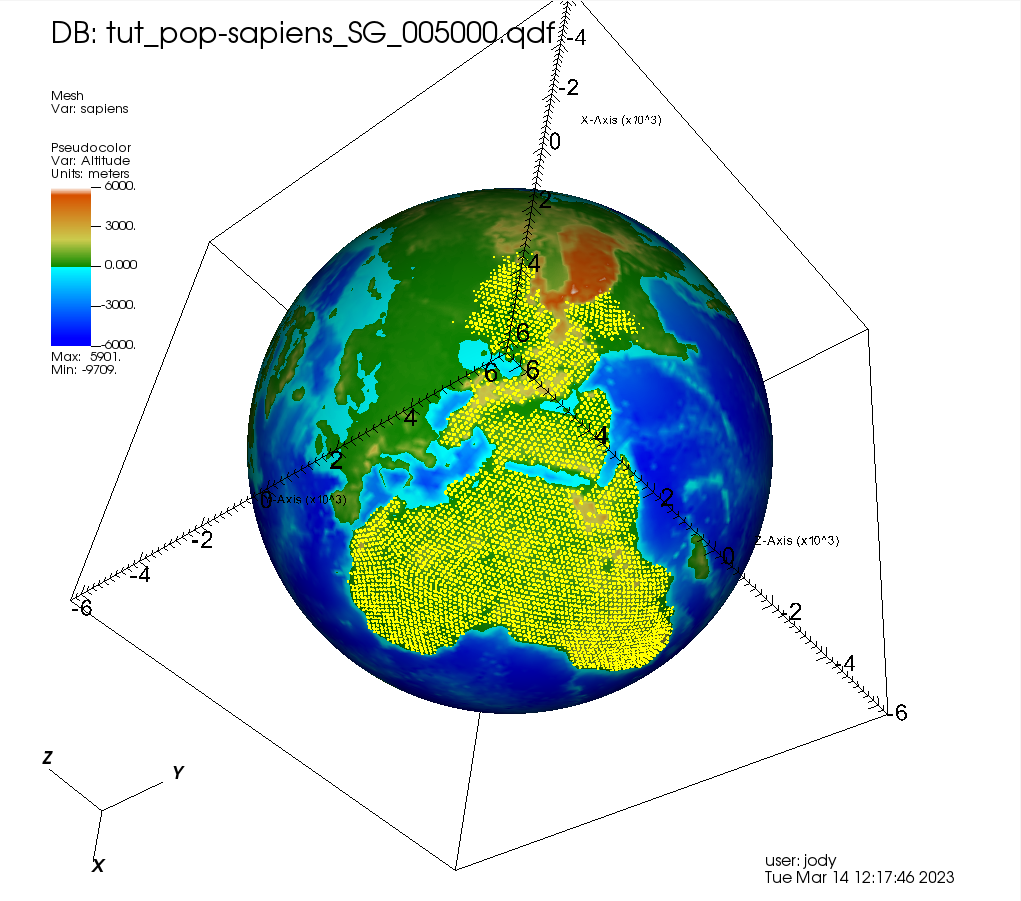
The next time you start VisIt you shoud see “geo2.ct” in the pseudocolor plot’s color tables.
When using geo2 the range should be symmetric around 0 (thus the values “-6000” and “6000” above), i.e. the value 0 should be in the exact middle between the two extremes. This must be the case so that negative values (i.e. underwater cells) are colored in bluish hues, while positive values are drawn with greenish and brownish colors.